단백질 : 논문리뷰 : AlphaFold: Improved protein structure prediction using potentials from deep learning

Overall Summary

AlphaFold는 특히 free modelling case에서 단백질 구조 예측(protein structure prediction)에 있어 획기적인 발전을 이룬 새로운 deep-learning 기반 시스템입니다. 전체 L × L distogram을 예측하고 deep residual network를 사용하여, gradient descent로 protein-specific potential을 최적화함으로써, 복잡한 sampling이나 domain segmentation 없이 state-of-the-art accuracy를 달성합니다. 이 향상된 정확도는, 특히 실험적으로 결정된 상동 구조(homologous structures)가 없는 단백질에 대해, 단백질 기능 및 기능 장애를 이해하기 위한 새로운 가능성을 열어줍니다. 단백질 과학(protein science) 및 crystallography의 molecular replacement에 도움이 될 수 있습니다.

쉬운 설명

AlphaFold는 단백질의 3차원 구조를 예측하는 새로운 딥러닝 시스템입니다. 기존 방법들과 달리, 단순히 아미노산 간의 "접촉" 여부만 예측하는 것이 아니라, 모든 아미노산 쌍 사이의 거리 분포를 정확하게 예측합니다. 마치 단백질의 상세한 "지도"를 그리는 것과 같습니다. 이 "지도" 정보를 바탕으로 단백질 구조를 나타내는 "에너지 함수"를 만들고, 경사 하강법(gradient descent)이라는 간단한 최적화 방법을 사용하여 에너지가 가장 낮은, 즉 가장 안정적인 구조를 찾아냅니다. 복잡한 시뮬레이션이나 여러 조각(domain)으로 나누는 과정 없이 전체 단백질을 한 번에 모델링하여 정확도를 크게 향상시켰습니다.

 

 

 

 

AlphaFold: Improved protein structure prediction using potentials from deep learning 학습 노트 (한국어 기반)

Purpose of the Paper

• Problem: 기존의 단백질 구조 결정(protein structure determination) 실험 방법들은 어렵고 시간이 오래 걸립니다. 전통적인 계산 방법들은 발전하고 있지만, 여전히 정확도가 부족하며, 특히 상동 서열(homologous sequences)이 적은 단백질(free modelling)의 경우 더욱 그렇습니다.
• Goal: 단순 contact prediction을 넘어, 잔기간 거리(inter-residue distance)를 정확하게 예측할 수 있는 deep learning 시스템을 개발하는 것입니다. 이 정보를 사용하여 복잡한 sampling procedure 없이 정확한 구조를 찾기 위해 최적화할 수 있는, 단백질 특이적 potential(protein-specific potential)을 구성합니다. Free modelling의 성능을 비약적으로 향상시키는 것을 목표로 합니다.
• Novel Approach: 새로운 deep-learning 기반 단백질 구조 예측 시스템을 도입합니다. Neural network를 사용하여 protein-specific potential을 구성하고, 간단한 gradient descent algorithm으로 최적화 합니다.

Key Contributions

• Distance Prediction: Deep residual convolutional neural network가 단순 contact뿐만 아니라, 모든 잔기 쌍 사이의 거리 분포(distribution of distances) 를 정확하게 예측합니다. 이 distogram은 contact map보다 더 자세한 구조 정보를 제공합니다.
• Protein-Specific Potential: 예측된 거리 분포(distance distributions), torsion angle 예측, 그리고 Rosetta의 van der Waals term을 결합하여 부드럽고 미분 가능한 potential을 구성합니다.
• Gradient Descent Optimization: 단백질 구조는 복잡한 sampling method(e.g. simulated annealing) 없이, 간단한 gradient descent algorithm (L-BFGS)을 사용하여 protein-specific potential을 직접 최적화함으로써 구현됩니다.
• End-to-End Optimization: 전체 단백질 chain을 동시에 최적화하여, 오류가 발생하기 쉬운 domain segmentation을 피합니다.
• 각 contribution의 Novelty:
  • Distogram 사용.
  • Protein-specific potential 구성.
  • End-to-end optimization으로 error-prone domain segmentation 회피.

Experimental Highlights

• CASP13 Performance: AlphaFold는 CASP13 blind assessment에서, 특히 free modelling (FM) category에서 다른 모든 방법보다 훨씬 높은 정확도를 달성했습니다.
  • AlphaFold는 43개 FM domain 중 24개에 대해 높은 정확도의 구조(TM-score ≥ 0.7)를 생성한 반면, 차순위 방법은 43개 중 14개였습니다.
• Distance Prediction Accuracy: 예측된 거리 분포(predicted distance distributions)는 실제 거리(true distances)와 매우 일치하며, 네트워크의 불확실성 추정(예측된 분포의 standard deviation)은 예측 정확도와 상관 관계가 있습니다.
• Potential Optimization: Gradient descent는 구성된 potential을 효과적으로 최소화하여 높은 TM-score를 갖는 구조를 만듭니다. 수백 번의 반복만으로도 수렴(convergence)하기에 충분합니다.
• Datasets:
  • Training: Protein Data Bank (PDB)의 non-redundant domain. CATH 35% sequence similarity cluster를 사용하여 필터링.
  • Test: CASP13 target 및 training set의 subset (상동 superfamily 당 단일 domain).
• Metrics: TM-score, GDT_TS, RMSD, lDDT, distogram lDDT (DLDDT).
• Baselines:
  • CASP13에 참여한 다른 그룹.
  • 최상위 contact prediction method (498: RaptorX-Contact, 032: TripletRes).
  • Potential의 다른 구성 요소를 제거하는 ablation study.
• Key Results:
  • Fig. 1a, 1b, 1c: CASP13에서 AlphaFold의 우수한 성능을 보여줍니다.
  • Fig. 3e, 3f: 거리 예측의 정확도와 보정된 불확실성(calibrated uncertainty)을 보여줍니다.
  • Fig. 4a: Distogram 정확도와 최종 구조 정확도 간의 상관 관계.
  • Fig. 4b: Distance potential의 중요성을 보여주는 ablation study.
  • Fig. 2e: Gradient descent 반복 횟수에 따른 평균 TM-score.
  • Fig 8b: DLIDDT12 vs effective number of sequences.
  • Fig 8c: 구성요소의 ablation study.

Limitations and Future Work

• Limitations:
  • Free modelling 예측은 여전히 실험 구조의 정확도에 거의 도달하지 못합니다.
  • AlphaFold의 FM 성능은 전례가 없지만, 여전히 template-based modelling (TBM) target에 비해 FM target의 정확도가 낮습니다.
  • Domain segmentation은 피하지만, 매우 긴 chain (예: T0999)은 여전히 homology 기반 수동 segmentation이 필요할 수 있습니다.
• Future Work:
  • 단백질 과학의 모든 영역에 도움이 되도록 방법을 더욱 발전시키는 것.
  • 네트워크가 예측을 수행하는 메커니즘을 탐구 (interpretability).
  • 예측된 구조를 단백질 기능에 대한 자세한 이해에 안정적으로 사용할 수 있도록 정확도를 향상시키는 것.
  • FM과 TBM 예측 간의 정확도 격차를 해결.

 

 

Abstract

Amino acid sequence로부터 protein의 3차원 shape를 결정하는 데 Protein structure prediction을 사용할 수 있습니다. 이 문제는 protein의 structure가 그 function을 크게 결정하기 때문에 근본적으로 중요합니다. 그러나 protein structure는 실험적으로 결정하기 어려울 수 있습니다. 최근 genetic information을 활용하여 상당한 진전이 이루어졌습니다. Homologous sequences의 covariation을 분석하여 어떤 amino acid residues가 contact 상태인지 추론할 수 있으며, 이는 protein structure prediction에 도움이 됩니다. 여기에서 우리는 neural network를 train하여 residue 쌍 사이의 거리에 대한 정확한 predictions를 수행할 수 있음을 보여줍니다. 이 predictions는 contact predictions보다 structure에 대한 더 많은 information을 전달합니다.

이 information을 사용하여 protein의 shape를 정확하게 설명할 수 있는 potential of mean force를 구성합니다. 우리는 결과 potential이 복잡한 sampling 절차 없이 간단한 gradient descent algorithm으로 optimized되어 structure를 generate할 수 있음을 발견했습니다.

AlphaFold라고 명명된 결과 system은 높은 accuracy를 달성하며, 심지어 homologous sequences가 더 적은 sequences에 대해서도 그러합니다. 최근의 Critical Assessment of Protein Structure Prediction (CASP13) - 이 분야의 state of the art에 대한 blind assessment - 에서 AlphaFold는 43개의 free modelling domains 중 24개에 대해 high-accuracy structures (template modelling (TM) scores 0.7 이상)를 생성한 반면, sampling과 contact information을 사용한 다음으로 가장 우수한 method는 43개 domains 중 14개에 대해서만 그러한 accuracy를 달성했습니다.

AlphaFold는 protein-structure prediction에서 상당한 진전을 나타냅니다. 우리는 이러한 accuracy 향상이 특히 homologous proteins에 대한 structure가 실험적으로 결정되지 않은 경우에 protein의 function과 malfunction에 대한 insights를 가능하게 할 것으로 기대합니다.

 

 

 

Introduction

Proteins은 대부분의 생물학적 과정의 핵심입니다. protein의 기능은 그 structure에 의존하기 때문에 protein structure를 이해하는 것은 수십 년 동안 생물학에서 큰 과제였습니다. 여러 experimental structure determination techniques가 개발되고 accuracy가 향상되었지만, 여전히 어렵고 시간이 많이 걸립니다. 그 결과, 수십 년 동안 이론적 연구를 통해 아미노산 sequence로부터 protein structure를 predict하려는 시도가 있었습니다.

CASP는 accuracy의 benchmark progress를 위해 structure prediction community에서 2년마다 실행하는 blind protein structure prediction assessment입니다. 2018년, AlphaFold는 CASP13에 참가한 전 세계 97개 그룹에 합류했습니다. 각 그룹은 experimentally determined structure가 격리된 84개의 protein sequence 각각에 대해 최대 5개의 structure prediction을 제출했습니다. Assessor는 scoring을 위해 protein을 104개의 domain으로 나누고, 각 domain을 template-based modelling (TBM, 유사한 sequence를 가진 protein이 known structure를 갖고, 해당 homologous structure가 sequence difference에 따라 modified되는 경우)에 적합하거나 free modelling (FM, homologous structure를 사용할 수 없는 경우)이 필요한 것으로 분류했으며, 중간 (FM/TBM) category도 있습니다.

Figure 1a는 AlphaFold가 다른 어떤 system보다 high accuracy로 더 많은 FM domain을 predict하며, 특히 0.6-0.7 TM-score 범위에서 그러함을 보여줍니다. 0과 1 사이의 값을 갖는 TM score는 제안된 structure의 overall (backbone) shape이 native structure와 일치하는 정도를 측정합니다. assessor는 98개 참가 그룹을 category별로 분리된 structure의 summed, capped z-score로 순위를 매겼습니다. AlphaFold는 FM category (best-of-five)에서 52.8의 summed z-score를 달성한 반면, 다음으로 가장 가까운 그룹 (322)은 36.6을 기록했습니다. FM 및 TBM/FM category를 합치면 AlphaFold는 68.3점을, 다음 그룹은 48.2점을 기록했습니다. AlphaFold는 이전에 알려지지 않은 fold를 high accuracy로 predict할 수 있습니다 (Fig. 1b). template을 사용하지 않고 FM techniques만 사용했음에도 불구하고, AlphaFold는 assessor의 공식 0-capped z-score에 따라 TBM category에서도 좋은 성적을 거두어 top-one model에서 4위, best-of-five models에서 1위를 차지했습니다. AlphaFold accuracy의 대부분은 distance prediction의 accuracy 덕분이며, 이는 해당 contact prediction의 high precision에서 분명하게 드러납니다 (Fig. 1c 및 Extended Data Fig. 2a).

지금까지 가장 성공적인 FM approaches는 fragment assembly에 의존했습니다. 이러한 approaches에서는 Protein Data Bank (PDB)에서 추출된 summary statistics에서 파생된 statistical potential을 minimize하는 simulated annealing과 같은 stochastic sampling process를 통해 structure가 생성됩니다. fragment assembly에서는 structure hypothesis가 반복적으로 modified되는데, 일반적으로 potential을 낮추는 change는 유지하면서 short section의 shape을 변경하여 ultimately low potential structure로 이어집니다. Simulated annealing은 수천 번의 이러한 move가 필요하며, low-potential structure를 잘 coverage하기 위해 여러 번 반복해야 합니다.

최근 몇 년 동안 structure prediction의 accuracy는 related sequences 집합에서 발견되는 evolutionary covariation data를 사용하여 향상되었습니다. target sequence와 유사한 sequence는 DNA sequencing에서 파생된 large datasets of protein sequences를 searching하고 target sequence에 aligned하여 multiple sequence alignment (MSA)를 generate함으로써 발견됩니다. MSA의 sequence에서 두 아미노산 residue 위치의 correlated change는 어떤 residue가 contact에 있을 수 있는지 추론하는 데 사용될 수 있습니다. Contacts는 일반적으로 2개의 residue의 β-carbon atom이 서로 8Å 이내에 있을 때 발생하는 것으로 defined됩니다. neural networks를 포함한 여러 methods가 MSA에서 computed된 features를 기반으로 한 쌍의 residue가 contact 상태일 probability를 predict하는 데 사용되었습니다. Contact predictions은 predicted contacts를 더 많이 만족시키는 structure로 folding process를 guide하기 위해 statistical potential을 modifying하여 structure predictions에 incorporated됩니다. 다른 studies에서는 특히 distance geometry approaches를 위해 residue 사이의 distance prediction을 사용했습니다. covariation features가 없는 Neural network distance predictions은 evolutionary pairwise distance-dependent statistical potential을 만드는 데 사용되었으며, 이는 structure hypotheses의 순위를 매기는 데 사용되었습니다. 또한, QUARK pipeline은 TBM을 위해 template-based distance-profile restraint를 사용했습니다.

이 연구에서는 protein structure prediction에 대한 deep-learning approach를 제시하며, 그 단계는 Fig. 2a에 illustrated되어 있습니다. 우리는 neural network (Fig. 2b)를 train하여 sequence가 주어지면 protein의 structure에 대한 accurate predictions을 하고, gradient descent (Fig. 2c)로 potential을 minimizing하여 structure 자체를 accurately predict함으로써 learned, protein-specific potential을 constructing할 수 있음을 보여줍니다. neural network predictions에는 backbone torsion angles와 residue 사이의 pairwise distances가 include됩니다. Distance predictions은 contact predictions보다 structure에 대한 더 specific information을 provide하고 neural network에 더 풍부한 training signal을 provide합니다. 많은 distances를 jointly predicting함으로써 network는 covariation, local structure 및 nearby residues의 residue identities를 respects하는 distance information을 propagate할 수 있습니다. predicted probability distributions는 결합되어 simple, principled protein-specific potential을 형성할 수 있습니다. 우리는 gradient descent를 사용하면 limited sampling만으로 이 protein-specific potential을 minimizes하는 torsion angles 집합을 쉽게 찾을 수 있음을 보여줍니다. 또한 whole chains를 simultaneously optimize할 수 있어, long proteins을 common practice인 independently modelled hypothesized domains으로 segment할 필요가 없음을 보여줍니다 (see Methods).

AlphaFold의 central component는 PDB structures에서 train되어 protein의 residue 쌍 ij의 Cβ atom 사이의 distances d_ij를 predict하는 convolutional neural network입니다. protein의 아미노산 sequence S의 representation과 해당 sequence의 MSA(S)에서 derived된 features를 basis으로, image-recognition tasks에 사용되는 것과 structure가 similar한 network는 Fig. 2b와 같이 L × L distance matrix의 모든 64 × 64 region에서 모든 ij 쌍에 대해 discrete probability distribution P(d_ij|S, MSA(S))를 predict합니다. entire distance map을 covers하는 이러한 predictions을 combining하여 constructed된 full set of distance distribution predictions을 distogram (distance histogram)이라고 합니다. 하나의 CASP protein인 T0955에 대한 example distogram predictions은 Fig. 3c, d에 shown되어 있습니다. distribution의 modes (Fig. 3c)는 true distances (Fig. 3b)와 closely match하는 것을 볼 수 있습니다. 한 residue (residue 29)까지의 모든 distances에 대한 example distributions은 Fig. 3d에 shown되어 있습니다. 우리는 distance predictions이 residue 사이의 true distance와 well correlate함을 발견했습니다 (Fig. 3e). 또한, network는 predictions의 uncertainty도 models합니다 (Fig. 3f). predicted distribution의 s.d.가 low이면 predictions은 more accurate합니다. 이것은 Fig. 3d에서도 evident하며, distance distribution에 대한 more confident predictions (higher peak 및 lower s.d. of the distribution)이 tend to be more accurate하며, true distance는 peak에 close합니다. Broader, less-confidently predicted distributions은 peak에 close하지 않을 때도 correct value에 probability를 assign합니다. distance predictions, 그리고 consequently contact predictions (Fig. 1c)의 high accuracy는 neural network의 design, training, data augmentation, feature representation, auxiliary losses, cropping 및 data curation의 factors combination에서 비롯됩니다 (see Methods).

distance predictions에 conform하는 structures를 generate하기 위해, 우리는 negative log probabilities에 spline을 fitting하고 모든 residue pairs에 대해 summing하여 smooth potential V_distance를 constructed했습니다 (see Methods). 우리는 모든 residues의 backbone torsion angles (φ, ψ)로 protein structures를 parameterized하고 protein geometry x = G(φ, ψ)의 differentiable model을 build하여 모든 residues i에 대한 Cβ coordinates, x_i를 compute하고, 따라서 inter-residue distances, d_ij = ||x_i - x_j||를 compute하고, 각 structure에 대해 V_distance를 φ and ψ의 function으로 express합니다. L residues를 가진 protein의 경우, 이 potential은 marginal distribution predictions에서 L² terms를 accumulates합니다. prior의 overrepresentation을 correct하기 위해, log domain에서 distance potential에서 reference distribution을 subtract합니다. reference distribution은 protein sequence와 independent하게 distance distributions P(d_ij|length)를 models하며, sequence 또는 MSA input features 없이 same structures에서 distance prediction neural network의 small version을 training하여 computed됩니다.

contact prediction network의 separate output head는 backbone torsion angles P(φ_i, ψ_i|S, MSA(S))의 discrete probability distributions을 predict하도록 trained됩니다. von Mises distribution을 fitting한 후, 이것은 potential에 smooth torsion modelling term, V_torsion을 add하는 데 used됩니다. Finally, steric clashes를 prevent하기 위해, van der Waals term을 incorporates하는 Rosetta의 V_{score2_smooth} score를 potential에 add합니다. 우리는 potential의 세 terms 각각에 대해 multiplicative weights를 used했지만, 어떤 weights combination도 equal weighting을 noticeably outperform하지 않았습니다.

combined potential V_total(φ, ψ)의 모든 terms가 (φ, ψ)의 differentiable functions이므로, gradient descent를 사용하여 이러한 variables에 대해 optimized될 수 있습니다. 여기서 우리는 L-BFGS를 use합니다. Structures는 P(φ_i, ψ_i|S, MSA(S))에서 torsion values를 sampling하여 initialized됩니다. Figure 2c는 potential을 minimizes하는 single gradient descent trajectory를 illustrates하며, 이 greedy optimization process가 어떻게 increasing accuracy와 large-scale conformation changes로 이어지는지 보여줍니다. secondary structure는 predicted torsion angle distributions에서 initialization에 의해 partly set됩니다. overall accuracy (TM score)는 quickly improve하고, 몇 백 steps의 gradient descent 후에 structure의 accuracy는 potential의 local optimum으로 converged됩니다.

우리는 sampled initializations에서 optimization을 repeated하여 low-potential structures의 pool을 만들고, 여기에서 further structure initializations가 sampled되며, added backbone torsion noise (‘noisy restarts’)를 통해 더 많은 structures가 pool에 added됩니다. only a few hundred cycles 후에 optimization은 converges되고 lowest potential structure가 best candidate structure로 chosen됩니다. Figure 2e는 gradient descent process의 multiple restarts에 걸쳐 best-scoring structures의 accuracy progress를 보여주며, 몇 번의 iterations 후에 optimization이 converged되었음을 보여줍니다. Noisy restarts는 predicted torsion distributions에서 sampling을 continue할 때보다 slightly higher TM score를 가진 structures를 found할 수 있게 합니다 (Extended Data Fig. 4에 shown된 test set에서 average 0.641 vs. 0.636).

Figure 4a는 distogram accuracy (distogram의 local distance difference test (lDDT)를 using measured; see Methods)가 final realized structures의 TM score와 well correlates함을 보여줍니다. Figure 4b는 potential construction을 changing하는 effect를 보여줍니다. distance potential을 entirely removing하면 0.266의 TM score가 나옵니다. adjacent bins를 averaging하여 distogram representation의 resolution을 six bins below로 reducing하면 TM score가 degrade됩니다. torsion potential, reference correction 또는 V_{score2_smooth}를 removing하면 accuracy가 only slightly degrade됩니다. Talaris2014 potential과 reference-corrected distance potential의 spline fit의 combination을 using하는 Rosetta를 이용한 final ‘relaxation’ (side-chain packing interleaved with gradient descent)은 side-chain atom coordinates를 adds하고, 0.007 TM score의 small average improvement를 yields합니다.

우리는 carefully designed deep-learning system이 inter-residue distances의 accurate predictions을 provide할 수 있고 protein structure를 represents하는 protein-specific potential을 construct하는 데 used될 수 있음을 보여줍니다. Furthermore, 우리는 이 potential이 gradient descent로 optimized되어 accurate structure predictions을 achieve할 수 있음을 보여줍니다. FM predictions은 rarely experimental structures의 accuracy에 approach하지만, CASP13 assessment는 AlphaFold system이 unprecedented FM accuracy를 achieves하고, 이 FM method가 templates를 using하지 않고 template-modelling approaches의 performance를 match할 수 있으며, biological insights를 provide하는 데 needed accuracy에 reach하기 시작했음을 보여줍니다 (see Methods). 우리는 우리가 described한 methods가 further developed되고 unknown structure의 sequences에 대해 more accurate predictions을 통해 protein science의 all areas에 benefit을 주기 위해 applied될 수 있기를 hope합니다.

 

 

 

 

AlphaFold Introduction Section: 정리 노트 (AI 연구자 대상)

핵심: AlphaFold는 protein structure prediction의 accuracy를 획기적으로 향상시킨 deep-learning system입니다. 기존 approaches와 근본적으로 다른 몇 가지 핵심적인 innovations를 도입합니다.

Key Innovations:

1. Distogram Prediction:
   • Residue 간의 contact를 직접 predicting하는 것(이진 분류) 대신, AlphaFold는 모든 residue 쌍 사이의 거리 분포를 predict합니다. 이 "distogram"은 protein의 3D structure에 대해 훨씬 풍부한 information을 제공합니다.
   • Convolutional neural network (image recognition에 사용되는 것과 유사)를 train하여 이러한 distogram을 predict하며, 아미노산 sequence와 MSA에서 파생된 features를 input으로 사용합니다.
   • Network는 거리를 predicting할 뿐만 아니라 prediction의 uncertainty도 modeling하여, 더욱 견고한 structure generation을 가능하게 합니다.
2. Learned, Protein-Specific Potential:
   • 예측된 distogram은 protein의 structure를 나타내는 부드러운 potential energy function (V_distance)으로 변환됩니다. 이 potential은 protein-specific하며, 각 protein에 대한 sequence와 MSA data로부터 직접 learn됩니다.
   • Network의 별도 output은 backbone torsion angles를 predict하며, 이는 potential (V_torsion)에도 통합됩니다.
   • Steric clashes는 Rosetta에서 파생된 항(V_{score2_smooth})을 추가하여 방지합니다.
3. Gradient Descent Optimization:
   • Stochastic sampling (예: simulated annealing)에 의존하는 기존 methods와 달리, AlphaFold는 gradient descent (구체적으로, L-BFGS)를 사용하여 potential energy function을 직접 optimize합니다.
   • Potential은 backbone torsion angles에 대해 differentiable하므로, gradient descent가 가능합니다. 이를 통해 conformational space를 효율적으로 탐색할 수 있습니다.
   • "Noisy restarts" (predicted torsion angle distributions에서 sampling하고 noise를 추가)를 사용하여 local optima에서 벗어납니다.
   • Optimization은 전체 chains에 대해 수행될 수 있으므로, domain segmentation이 필요하지 않습니다.
4. End-to-end, Differentiable Process:
   • Gradient descent를 통해 optimize하는 과정은 전체 chain을 동시에 진행할 수 있으며, hypothesized domains으로 나누어 진행할 필요가 없습니다.

Results:

• CASP13에서 AlphaFold는 free modelling (FM) category에서 다른 모든 methods를 크게 능가하여 전례 없는 accuracy를 달성했습니다.
• AlphaFold의 performance는 template-based modelling (TBM) category에서도 강력했지만, templates를 명시적으로 사용하지는 않습니다.

Impact: * High-accuracy protein structure, protein의 malfunction, unknown structure의 sequences에 대한 prediction 가능.

차별점 요약:

• Distogram prediction: Contact prediction보다 더 풍부한 structure representation을 제공합니다.
• Learned, protein-specific potential: Gradient descent를 통한 직접 optimization을 가능하게 합니다.
• Gradient descent optimization: Stochastic sampling보다 효율적입니다.
• End-to-end differentiable: Domain segmentation 없이 optimization을 가능하게 합니다.

---

쉬운 설명:

AlphaFold의 Introduction 섹션에서는 이 system이 기존의 protein structure prediction 방법들과 어떻게 다르고, 왜 더 좋은 성능을 내는지 설명하고 있습니다.

핵심은 AlphaFold가 "distogram"이라는 것을 predicting한다는 점입니다. 기존에는 단순히 두 아미노산 residue가 "가까이 있다/없다" (contact prediction)만 predicting했다면, AlphaFold는 모든 residue 쌍 사이의 거리 분포를 predicting합니다. 마치 건물 설계도에서 각 방 사이의 거리를 상세하게 표시하는 것과 같습니다.

이렇게 얻은 거리 information을 바탕으로, AlphaFold는 해당 protein만의 "potential energy"를 계산합니다. 이 potential energy는 protein이 어떤 모양일 때 가장 안정적인지를 나타내는 함수입니다. 마치 구슬이 굴러서 가장 낮은 지점에 멈추는 것처럼, AlphaFold는 이 potential energy를 가장 낮추는 protein 모양을 찾습니다.

이때 AlphaFold는 "gradient descent"라는 방법을 사용하는데, 이는 마치 경사진 산에서 가장 낮은 곳을 찾아 내려가는 것과 비슷합니다. 기존에는 무작위로 여기저기 탐색하는 방법(simulated annealing)을 사용했지만, AlphaFold는 훨씬 효율적으로 최적의 structure를 찾을 수 있습니다.

마지막으로, AlphaFold는 전체 protein을 한 번에 optimize할 수 있습니다. 기존에는 긴 protein을 여러 조각(domain)으로 나누어 따로따로 predicting해야 했지만, AlphaFold는 그런 과정 없이 전체를 한 번에 처리할 수 있습니다.

이러한 innovations 덕분에 AlphaFold는 CASP13이라는 대회에서 다른 모든 methods를 압도하고, protein structure prediction 분야에 큰 발전을 가져왔습니다.

 

 

Methods

Extended Data Figure 1a는 MSA construction, feature extraction, distance prediction, potential construction 및 structure realization에 관련된 단계를 보여줍니다.

Tools

CASP system과 후속 실험을 위해 다음과 같은 tools 및 dataset versions이 사용되었습니다: PDB 15 March 2018; CATH 16 March 2018; HHblits based on v.3.0-beta.3 (three iterations, E = 1 × 10^-3); HHpred web server; Uniclust30 2017-10; PSI-BLAST v.2.6.0 nr dataset (as of 15 December 2017) (three iterations, E = 1 × 10^-3); SST web server (March 2019); BioPython v.1.65; Rosetta v.3.5; PyMol 2.2.0 for structure visualization; TM-align 20160521.

Data

우리 models은 PDB에서 추출한 structures에 대해 trained됩니다. CATH 35% sequence similarity cluster representatives를 활용하여 non-redundant domains을 추출합니다. 이렇게 생성된 31,247개의 domains은 train 및 test sets (각각 29,427개와 1,820개의 proteins)로 분할되었으며, 동일한 homologous superfamily (CATH classification에서 H-level)의 모든 domains은 동일한 partition에 유지되었습니다. CASP11 및 CASP12의 FM domains의 CATH superfamilies도 training set에서 제외되었습니다. Test set에서, 여기에 제시된 결과에 사용된 377개의 domain subset을 만들기 위해 homologous superfamily 당 하나의 domain을 무작위로 선택했습니다. 이 set에 대한 accuracies는 CASP13 test domains보다 높습니다.

CASP13 submission results는 CASP13 결과 페이지에서 가져왔으며, CASP domain definitions에 의해 CASP13 PDB files에서 scored된 'all groups' chains에 대한 CASP13 dataset에 대한 추가 결과가 표시됩니다. Contact prediction accuracies는 AlphaFold가 CASP13 submissions에 사용한 distogram predictions과 비교하여 group 032 및 498 submissions (RR files 형식)에서 다시 계산되었습니다. Contact prediction probabilities는 각 distribution에서 8Å 미만의 probability mass를 합산하여 distograms에서 얻었습니다.

각 training sequence에 대해 Uniclust30 dataset에서 training sequence와 유사한 protein sequences를 검색하고 HHblits를 사용하여 aligned했으며, 반환된 MSA를 사용하여 각 residue에 대한 position-specific substitution probabilities와 covariation features (CCMpred와 유사한 regularized pseudo-likelihood-trained Potts model의 parameters)를 가진 profile features를 generate했습니다. CCMPred는 parameters의 Frobenius norm을 사용하지만, 우리는 이 norm (1 feature)과 raw parameters (484 features)를 모두 각 residue 쌍 ij에 대해 network에 제공합니다. 또한, network에 MSA의 gaps와 deletions을 명시적으로 나타내는 features를 제공합니다. Network가 얕은 MSA에 대한 predictions을 더 잘 수행할 수 있도록 하고, data augmentation의 한 형태로, MSA-based features를 computing하기 전에 HHblits MSA에서 sequences의 절반을 sample로 취합니다. 우리 training set에는 각 domain에 대해 10개의 이러한 samples가 포함되어 있습니다. PSI-BLAST를 사용하여 추가 profile features를 추출합니다.

Distance prediction neural network는 다음 input features를 사용하여 trained되었습니다 (features 수는 괄호 안에 표시).

• HHblits alignments 수 (scalar).
• Sequence-length features: 1-hot 아미노산 type (21 features); profiles: PSI-BLAST (21 features), HHblits profile (22 features), non-gapped profile (21 features), HHblits bias, HMM profile (30 features), Potts model bias (22 features); deletion probability (1 feature); residue index (residue number의 integer index, multi-segment domains을 제외하고 연속적이며, 5개의 least-significant bits와 scalar로 encoded됨).
• Sequence-length-squared features: Potts model parameters (484 features, Nesterov momentum 0.99를 사용하고 sequence reweighting 없이 500 iterations의 gradient descent로 fitted됨); Frobenius norm (1 feature); gap matrix (1 feature).

z-scores는 CASP13 assessors의 결과(http://predictioncenter.org/casp13/zscores_final.cgi?formula=assessors)에서%EC%97%90%EC%84%9C) 가져왔습니다.

Distogram prediction. Inter-residue distances는 deep neural network에 의해 predicted됩니다. Architecture는 deep two-dimensional dilated convolutional residual network입니다. 이전에는 contact prediction을 위해 1차원 embedding layers가 앞에 오는 2차원 residual network가 사용되었습니다. 우리 network는 전체적으로 2차원이며 dilated convolutions을 가진 220개의 residual blocks를 사용합니다. Extended Data Fig. 1b에 illustrated된 각 residual block은 3개의 batchnorm layers; 2개의 1 × 1 projection layers; 3 × 3 dilated convolution layer 및 exponential linear unit (ELU) nonlinearities를 interleave하는 sequence of neural network layers로 구성됩니다. Successive layers는 cropped region 전체에 information을 빠르게 propagation하기 위해 1, 2, 4, 8 pixels의 dilations을 통해 순환합니다. Final layer의 경우, position-specific bias가 사용되었으며, biases는 residue-offset (32로 제한) 및 bin number로 indexed되었습니다.

Network는 cross-entropy loss를 사용하는 stochastic gradient descent로 trained됩니다. Target은 residues의 Cβ atoms (또는 glycine의 경우 Cα) 사이의 거리를 quantification한 것입니다. 2–22 Å 범위를 64개의 동일한 bins으로 나눕니다. Network에 대한 input은 각 i,j feature가 i와 j 모두에 대한 1차원 features와 i,j에 대한 2차원 features의 concatenation인 2차원 array of features로 구성됩니다.

Individual training runs은 27개의 CASP11 FM domains을 validation set으로 사용하여 early stopping으로 cross-validated되었습니다. Models은 27개의 CASP12 FM domains에 대한 cross-validation으로 selected되었습니다.

Neural network hyperparameters

• 256 channels를 가진 4개의 blocks로 구성된 7 groups, dilations 1, 2, 4, 8을 순환.
• 128 channels를 가진 4개의 blocks로 구성된 48 groups, dilations 1, 2, 4, 8을 순환.
• Optimization: synchronized stochastic gradient descent
• Batch size: 8개의 GPU workers 각각에 4개의 crops batch.
• 0.85 dropout keep probability.
• Nonlinearity: ELU.
• Learning rate: 0.06.
• Auxiliary loss weights: secondary structure: 0.005; accessible surface area: 0.001. 이러한 auxiliary losses는 100,000 steps 후에 10배 감소되었습니다.
• Learning rate는 150,000, 200,000, 250,000 및 350,000 steps에서 50% 감소되었습니다.
• Training time: 600,000 steps 동안 약 5일.

Cropped distograms. Memory usage를 제한하고 overfitting을 방지하기 위해, network는 항상 distance matrix의 64 × 64 regions, 즉 64개의 연속 residues와 다른 64개의 연속 residues 그룹 사이의 pairwise distances에 대해 trained되고 tested되었습니다. 각 training domain에 대해, 전체 distance matrix는 겹치지 않는 64 × 64 crops으로 분할되었습니다. Off-diagonal crops을 training함으로써, 64 residues보다 더 멀리 떨어져 있는 residues 간의 interaction을 modelled할 수 있습니다. 각 crop은 두 개의 64-residue fragments의 juxtaposition을 나타내는 distance matrix로 구성되었습니다. 이전에 contact prediction에는 제한된 context window만 필요하다는 것이 밝혀졌습니다. Diagonal i = j에 가까운 distance predictions은 protein의 local structure에 대한 predictions을 encode하고, cropped region의 경우 distances는 crop의 i 및 j 범위로 표현되는 두 fragments의 local structure에 의해 결정됩니다. i 및 j 범위 모두에 해당하는 on-diagonal two-dimensional input features로 inputs를 augmenting하면 각 fragment의 structure와 그 사이의 distances를 predict하기 위한 추가 information을 제공합니다. Fragment structures를 잘 predicted할 수 있다면 (예를 들어, helices 또는 sheets로 확실하게 predicted되는 경우), fragments 사이의 단일 contact prediction은 다른 모든 쌍 사이의 distances를 강력하게 constrain합니다.

Domain이 training에 사용될 때마다 crops의 offset을 randomizing하면 단일 protein이 수천 개의 서로 다른 training examples를 generate할 수 있는 data augmentation 형태가 됩니다. 이는 atom coordinates에 ground-truth resolution에 비례하는 noise를 추가하여 target distances에 variation을 유발함으로써 더욱 강화됩니다. Data augmentation (MSA subsampling 및 coordinate noise)은 dropout과 함께 network가 training data에 overfitting되는 것을 방지합니다.

모든 L × L residue 쌍에 대한 distance distribution을 predict하기 위해, 많은 64 × 64 crops이 combined됩니다. Edge effects를 피하기 위해, 서로 다른 offsets을 가진 여러 개의 이러한 tilings이 생성되고 averaged되며, crop 중앙 근처의 predictions에 더 큰 가중치가 부여됩니다. Accuracy를 더욱 improve하기 위해, 약간 다른 hyperparameters로 독립적으로 trained된 4개의 개별 models의 ensemble에서 predictions을 averaged합니다. Extended Data Figure 2b, c는 3-domain CASP13 target인 T0990에 대한 true distances와 distogram predictions의 mode의 examples를 보여줍니다.

Network는 MSA의 profile과 covariation features를 모두 incorporating할 수 있는 풍부한 representation을 가지고 있으므로, network를 사용하여 secondary structure를 직접 predict할 수 있다고 주장합니다. Network의 penultimate layer의 2차원 activations을 i와 j에서 별도로 mean- 및 max-pooling함으로써, j와 i의 각 residue에 대해 DSSP로 computed된 8-class secondary structure labels를 predict하는 추가 1차원 output head를 network에 추가합니다. 결과 Q3 (three helix/sheet/coil classes 구분) predictions의 accuracy는 84%이며, 이는 state-of-the-art predictions와 비슷합니다. 각 residue의 상대 accessible surface area (ASA)도 predicted될 수 있습니다.

1차원 pooled activations는 또한 각 residue에 대해 독립적으로 marginal Ramachandran distributions, P(φ_i, ψ_i|S,MSA(S))를 10° (1,296 bins)로 approximated된 discrete probability distribution으로 predict하는 데 사용됩니다. 실제로 CASP13 동안 우리는 distograms, secondary structure 및 ASA를 predict하도록 trained된 network의 distograms를 사용했습니다. Torsion predictions은 distograms, secondary structure, ASA 및 torsions을 predict하도록 trained된 두 번째 유사한 network에서 가져왔는데, 이는 전자가 더 철저하게 validated되었기 때문입니다.

Extended Data Figure 3b는 distograms의 accuracy에서 중요한 factor가 MSA의 effective number of sequences인 N_eff임을 보여줍니다 (이전에 contact prediction systems에서 발견된 바와 같이). 이것은 MSA에서 발견된 sequences의 수이며, 62% sequence identity level에서 redundancy를 discounting한 다음 target의 residues 수로 나눈 값이며, MSA의 covariation information의 양을 나타냅니다.

Distance potential. Distogram probabilities는 discrete distance bins에 대해 estimated되므로, differentiable potential을 construct하기 위해, distribution은 cubic spline으로 interpolated됩니다. Final bin은 22 Å 이상의 모든 distances에서 probability mass를 accumulates하고, 더 큰 distances는 정확하게 predict하기 어렵기 때문에, potential은 18 Å (cross-validation으로 결정)까지만 fitted되었으며, 그 이후에는 constant extrapolation이 적용되었습니다. Extended Data Figure 3c (bottom)은 distance histograms의 resolution을 변경하는 것이 structure accuracy에 미치는 영향을 보여줍니다.

Reference distribution을 predict하기 위해, 유사한 model이 동일한 dataset에서 trained됩니다. Reference distribution은 sequence에 conditioned되지 않지만, distances를 predicting하는 atoms를 고려하기 위해, residue가 glycine (Cα atom)인지 아닌지 (Cβ)와 protein의 전체 길이를 나타내는 이진 feature δ_αβ를 제공합니다.

Distance potential은 모든 residue 쌍 i, j에 대해 합산된 distances의 negative log likelihood에서 생성됩니다 (Supplementary equation (1)). Reference state를 사용하면, 이것은 full conditional model과 background model (Supplementary equation (2))에서 distances의 log-likelihood ratio가 됩니다.

Torsions은 predicted torsion distributions에서 negative log likelihood로 modelled됩니다. 우리는 marginal distribution predictions을 가지고 있으며, 각 prediction은 multimodal일 수 있으므로, torsions을 jointly optimize하기 어려울 수 있습니다. 모든 probability mass를 unify하기 위해, multimodal distributions의 modelling fidelity를 희생하여, marginal predictions에 unimodal von Mises distribution을 fitted했습니다. 이 potential은 모든 residues i에 대해 합산되었습니다 (Supplementary equation (3)).

마지막으로, steric clashes를 방지하기 위해, Rosetta의 V_{score2_smooth}를 사용하여 van der Waals term을 도입했습니다. Extended Data Figure 3c (top)은 potential의 다른 terms이 structure prediction의 accuracy에 미치는 영향을 보여줍니다.

Structure realization by gradient descent.

구성된 potential을 minimize하는 structures를 realize하기 위해, torsion angles (φ, ψ)의 function으로 backbone atom coordinates를 제공하는 ideal protein backbone geometry의 differentiable model, x = G(φ, ψ)를 만들었습니다. Minimize할 전체 potential은 distance, torsion 및 score2_smooth의 합입니다 (Supplementary equation (4)). 이러한 potentials가 동일한 scale을 갖는다는 보장은 없지만, terms에 대한 scaling parameters가 도입되었고 CASP12 FM domains에 대한 cross-validation으로 선택되었습니다. 실제로 모든 terms에 대해 동일한 가중치를 부여하는 것이 가장 좋은 결과를 가져오는 것으로 나타났습니다.

V_total의 모든 term은 torsion angles에 대해 differentiable하므로, predicted torsion marginals에서 sampled될 수 있는 initial set of torsions φ, ψ가 주어지면, L-BFGS와 같은 gradient descent algorithm을 사용하여 V_total을 minimize할 수 있습니다. Optimized structure는 initial conditions에 따라 달라지므로, 서로 다른 initializations로 optimization을 여러 번 반복합니다. 20개의 가장 낮은 potential structures의 pool이 유지되고, 일단 가득 차면, trajectories의 90%를 backbone torsions에 30° noise를 추가하여 initialize합니다 (나머지 10%는 여전히 predicted torsion distributions에서 sampled됨). CASP13에서는 각 chain에 대해 5,000번의 optimization runs를 얻었습니다. Figure 2c는 protein 당 restarts 횟수에 따른 TM score의 변화를 보여줍니다. 더 긴 chains은 optimize하는 데 시간이 더 오래 걸리므로, 이 작업 부하는 (50 + L)/2 병렬 workers에 분산되었습니다. Extended Data Figure 4는 predicted marginal distributions에서 시작 torsions를 sampling하는 것과 이전 structures의 pool에서 restarting하는 것을 비교하면서, 계산 시간에 따른 유사한 곡선을 보여줍니다.

Accuracy (정확도)

최종 structures를 experimentally determined structures와 비교하여 TM score, GDT_TS (global distance test, total score), r.m.s.d.와 같은 metrics를 사용하여 accuracy를 측정합니다. 이러한 모든 accuracy measures는 candidate structure와 experimental structure 간의 geometric alignment가 필요합니다. Alignment가 필요 없는 대안적인 accuracy measure는 lDDT이며, 이는 15 Å 미만의 native pairwise distances D_ij (sequence offsets ≥ r residues) 중 candidate structure에서 realized된 것(d_ij)의 비율을 true value의 tolerance 내에서 측정하고, 0.5, 1, 2, 4 Å의 tolerances에 대해 평균을 냅니다 (stereochemical checks 없이) (Supplementary equation (5) 참조).

Distogram이 pairwise distances를 predict하므로, Supplementary equation (6)과 같이 distograms의 probabilities에서 직접 computed되는 lDDT와 유사한 measure인 distogram lDDT (DLDDT)를 도입할 수 있습니다. Sequence에서 가까운 residues 간의 distances는 종종 짧고, predict하기 쉽고, 전체 fold topology를 결정하는 데 중요하지 않기 때문에, r = 12로 설정하여 sequence separation이 12 이상인 distances만 고려했습니다. 우리는 Cβ distances를 predict하기 때문에, 이 연구에서는 Cβ distances를 사용하여 lDDT와 DLDDT를 모두 computed했습니다. Extended Data Figure 3a는 DLDDT₁₂가 realized structures의 lDDT₁₂와 높은 상관관계 (CASP13의 경우 Pearson's r = 0.92)를 갖는다는 것을 보여줍니다.

Full chains without domain segmentation (도메인 분할 없는 전체 체인)

길이 L의 proteins을 residue 당 두 개의 torsion angles로 parameterizing하면, structures 공간의 차원은 2L로 증가합니다. 따라서 큰 proteins의 structures를 searching하는 것은 훨씬 더 어려워집니다. 전통적으로 이 문제는 더 긴 protein chains을 독립적으로 fold되는 조각(domains이라고 함)으로 분할하여 해결했습니다. 그러나 sequence만으로 domain segmentation하는 것은 그 자체로 어렵고 오류가 발생하기 쉽습니다. 이 연구에서는 domain segmentation을 피하고 전체 chains을 folded했습니다. 일반적으로 MSA는 주어진 domain segmentation을 기반으로 합니다. 그러나 우리는 sliding window approach를 사용하여 full-chain MSA를 compute하여 baseline full-sequence distogram을 predict했습니다. 그런 다음 chain의 subsequences에 대한 MSA를 computed했으며, 크기가 64, 128, 256인 windows를 64의 배수로 offsets하여 시도했습니다. 이러한 각 MSA는 full-chain distogram의 on-diagonal square에 해당하는 개별 distogram을 생성했습니다. 우리는 이러한 모든 distograms을 함께 averaged하고, MSA의 sequences 수에 따라 가중치를 부여하여 많은 alignments를 찾을 수 있는 영역에서 더 정확한 평균 full-chain distogram을 생성했습니다. CASP13 assessment의 경우, 전체 chains은 V_Talaris2014 + 0.2 V_distance의 potential (가중치는 cross-validation으로 결정)을 사용하여 Rosetta relax로 relaxed되었으며, 모든 systems의 submissions은 이 potential을 기반으로 순위가 매겨졌습니다.

CASP13 results (CASP13 결과) CASP13의 경우, 5개의 AlphaFold submissions는 3개의 서로 다른 systems에서 가져온 것이며, 모두 neural network distance predictions를 기반으로 하는 potentials를 사용했습니다. 여기에 설명되지 않은 systems은 별도의 논문에 설명되어 있습니다. T0975 이전에는 simulated annealing과 fragment assembly를 기반으로 하는 두 개의 systems (40-bin distance distributions 사용)이 사용되었습니다. T0975부터는 새로 trained된 64-bin distogram predictions가 사용되었고, 여기에 설명된 gradient descent system (3개의 독립적인 runs)과 fragment assembly systems 중 하나 (5개의 독립적인 runs)에 의해 structures가 generated되었습니다. 5개의 submissions는 이러한 8개의 structures (각 독립적인 run에서 생성된 가장 낮은 potential structure)에서 선택되었으며, 첫 번째 submission (top-one)은 gradient descent로 생성된 가장 낮은 potential structure였습니다. 나머지 4개의 submissions는 4개의 가장 좋은 다른 structures였으며, 5번째는 2, 3, 4번째 위치에 선택되지 않은 경우 gradient descent structure였습니다. T0999에 대한 모든 submissions는 gradient descent로 generated되었습니다. Extended Data Figure 5a는 T0975 이전 targets에 대한 단일 run의 gradient descent로 generated된 'back-fill' structures와 비교하여 각 submission에 사용된 methods를 보여줍니다. Extended Data Figure 5b는 CASP에서 나중에 사용된 gradient descent method가 각 category에서 fragment assembly method보다 더 나은 performance를 보였다는 것을 보여줍니다. Extended Data Figure 5c는 FM 및 FM/TBM domains에 대한 AlphaFold submissions의 accuracy를 다음으로 가장 좋은 group 322와 비교합니다. CASP13 FM의 assessors는 전문가의 visual inspection을 사용하여 각 target에 대한 최상의 submissions를 선택했으며, AlphaFold가 다음으로 가장 좋은 그룹보다 거의 두 배나 많은 최상의 models을 가지고 있음을 발견했습니다.

Biological relevance of AlphaFold predictions (AlphaFold 예측의 생물학적 관련성)

Predicted structures는 fold shape를 일반적으로 이해하는 것부터 binding regions의 상세한 side-chain configurations를 이해하는 것까지, 모두 다른 accuracy requirements를 가진 광범위한 용도로 사용됩니다. Contact predictions만으로도 protein을 불안정하게 만들기 위해 mutations을 target하는 것과 같이 생물학적 insights를 안내할 수 있습니다. Figure 1c 및 Extended Data Figure 2a는 AlphaFold의 contact predictions의 accuracy가 state-of-the-art predictions의 accuracy를 초과한다는 것을 보여줍니다. Extended Data Figures 6-8에서는 AlphaFold의 accuracy improvements가 더 정확한 기능 해석 (Extended Data Figure 6)으로 이어진다는 것을 보여주는 추가 결과를 제시합니다. protein–protein interactions에 대한 더 나은 interface prediction (Extended Data Figure 7); 더 나은 binding pocket prediction (Extended Data Figure 8) 및 crystallography에서 개선된 molecular replacement.

지금까지는 template-based predictions만이 가장 정확한 predictions을 제공할 수 있었습니다. AlphaFold는 templates를 사용하지 않고 TBM과 일치할 수 있고, 어떤 경우에는 다른 methods보다 성능이 우수하지만 (예: T0981-D5, 72.8 GDT_TS, 및 T0957s1-D2, 88.0 GDT_TS, AlphaFold의 top-one model이 다른 어떤 top-one submission보다 12 GDT_TS 더 나은 두 개의 TBM-hard domains), FM targets에 대한 accuracy는 여전히 TBM targets에 대한 accuracy보다 뒤떨어지며, 어려운 structures에 대한 자세한 이해를 위해 여전히 의존할 수 없습니다. Molecular replacement에 대한 CASP13 TBM predictions의 performance에 대한 분석에서, 다른 연구에서는 AlphaFold predictions (B-factors 없이, raw coordinates)이 다른 어떤 그룹보다 약간 더 큰 log-likelihood gain을 가져왔다고 보고했으며, 이는 이러한 개선된 structures가 X-ray crystallography의 phasing을 지원할 수 있음을 나타냅니다.

Interpretation of distogram neural network (distogram 신경망 해석)

우리는 deep distance prediction neural network가 high accuracy를 달성한다는 것을 보여주었지만, network가 어떻게 distance predictions에 도달하는지, 특히 model에 대한 inputs가 최종 prediction에 어떤 영향을 미치는지 이해하고 싶습니다. 이것은 folding mechanisms에 대한 우리의 이해를 향상시키거나 model 개선을 제안할 수 있습니다. 그러나 deep neural networks는 inputs의 복잡한 비선형 functions이므로, 이 attribution problem은 어렵고, 불완전하게 지정되었으며, 진행 중인 연구 주제입니다. 그럼에도 불구하고, 이러한 분석을 위한 여러 가지 methods가 있습니다. 여기서 우리는 trained distogram network에 Integrated Gradients를 적용하여 network의 특정 거리에 대한 predictions에 영향을 미치는 input features의 위치를 나타냅니다.

Extended Data Figure 9에서는 T0986s2에서 선택된 I, J output 쌍에 대해 합산된 절대 Integrated Gradient, Σ_c|S^I,J_i,j,c| (Supplementary equations (7)-(9)에 정의됨)의 plots을 보여줍니다. Extended Data Figure 10에서는 각 output 쌍에 대한 상위 10개의 가장 높은 attribution input 쌍이 AlphaFold의 top-one predicted structure 위에 표시됩니다. Attribution maps는 희소하고 고도로 구조화되어 protein의 predicted geometry를 밀접하게 반영합니다. 제시된 4개의 in-contact 쌍 (1, 2, 3, 5)의 경우, 가장 높은 attribution 쌍은 모두 output 쌍 중 하나 또는 둘 다가 속한 secondary structure 내부 또는 사이의 쌍입니다. 1에서, helix residues는 helix의 양쪽 끝을 따르는 strands 사이의 연결뿐만 아니라 중요하며, 이는 helix의 변형을 나타낼 수 있습니다. 2에서, 가장 중요한 residue 쌍은 모두 동일한 두 strands를 연결하는 반면, 3에서는 inter-strand 쌍과 strand residues의 혼합이 가장 두드러집니다. 5에서, 가장 중요한 쌍은 strand와 helix에 대한 인접한 secondary structure elements의 packing을 포함합니다. Non-contacting 쌍 4의 경우, 가장 중요한 input 쌍은 predicted protein structure에서 I와 J 사이에 기하학적으로 있는 residues입니다. 또한, 대부분의 high-attribution input 쌍은 그 자체가 contact 상태입니다.

Network는 input에서 structure를 사용할 수 없는 상태에서 spatial geometry를 predicting하는 task를 수행하므로, 이러한 interaction patterns는 network가 중요한 interactions를 발견하고 관련 residues에서 information을 channeling하여 최종 prediction을 refine하기 위해 중간 predictions를 사용하고 있음을 나타냅니다.

Reporting summary (보고 요약)

Research design에 대한 추가 information은 이 논문에 링크된 Nature Research Reporting Summary에서 확인할 수 있습니다.

 

AlphaFold Methods Section: 정리 노트 (AI 연구자 대상)

핵심: AlphaFold는 protein structure prediction을 위해 end-to-end differentiable한 pipeline을 구축했습니다. 이 pipeline은 크게 (1) distogram prediction, (2) potential construction, (3) structure realization의 세 단계로 구성됩니다.

Key Components:

1. MSA Construction and Feature Extraction:
   • HHblits, PSI-BLAST 등 다양한 tools을 사용하여 target sequence에 대한 MSA를 구축합니다.
   • MSA로부터 profile features (position-specific substitution probabilities)와 covariation features (Potts model parameters)를 추출합니다.
   • Data augmentation을 위해 MSA subsampling을 사용합니다.
   • Sequence 자체의 features (1-hot encoding, residue index 등)도 활용합니다.
2. Distogram Prediction (Neural Network):
   • 핵심 component는 deep two-dimensional dilated convolutional residual network입니다.
     • 220 residual blocks with dilated convolutions (dilations 1, 2, 4, 8 cycling).
     • Input: sequence features, MSA-derived features (concatenated).
     • Output: distance distribution (distogram) for every pair of residues (64 bins for 2-22 Å).
   • Cropped training: Memory 제약과 overfitting 방지를 위해 64x64 regions of the distance matrix를 사용합니다.
   • Data augmentation: Random cropping, coordinate noise 추가.
   • Auxiliary losses: Secondary structure, accessible surface area (ASA) prediction.
   • Ensemble: 여러 models의 predictions을 averaging하여 accuracy 향상.
3. Potential Construction:
   • Distogram probabilities를 cubic spline으로 interpolation하여 differentiable potential (V_distance)을 생성합니다.
   • Reference distribution을 subtract하여 prior를 보정합니다.
   • Backbone torsion angles에 대한 marginal distributions를 predict하고, von Mises distribution으로 fitting하여 torsion potential (V_torsion)을 추가합니다.
   • Rosetta의 V_{score2_smooth}를 사용하여 steric clashes를 방지합니다.
4. Structure Realization (Gradient Descent):
   • Differentiable model of ideal protein backbone geometry (x = G(φ, ψ))를 사용하여 torsion angles로부터 atom coordinates를 계산합니다.
   • Total potential (V_total = V_distance + V_torsion + V_{score2_smooth})을 gradient descent (L-BFGS)로 minimize합니다.
   • Multiple initializations and "noisy restarts"를 사용하여 local optima 문제를 완화합니다.
   • Full chains are folded without domain segmentation.
5. Interpretation (해석)
   • Integrated Gradients를 활용하여 distogram 예측에 영향을 주는 input feature를 파악.

차별점 요약:

• End-to-end differentiable pipeline: Distogram prediction부터 structure realization까지 모든 과정이 differentiable하여 gradient descent를 통한 optimization이 가능합니다.
• Deep two-dimensional dilated convolutional residual network: Distogram prediction을 위한 강력한 architecture.
• Cropped training and data augmentation: Memory 효율성과 generalization 성능 향상.
• Learned, protein-specific potential: Sequence와 MSA data로부터 직접 potential을 learn합니다.
• Full-chain folding: Domain segmentation 없이 전체 chain을 folding.
• 해석 : Integrated Gradients를 활용해 distogram prediction에 영향을 주는 input feature 파악.

---

쉬운 설명:

AlphaFold의 Methods 섹션에서는 이 system이 protein structure를 predicting하기 위해 어떤 tools과 techniques를 사용하는지 자세히 설명합니다.

크게 세 단계로 나눌 수 있습니다.

1. Distogram 만들기:
   • 우선, target protein과 sequence가 비슷한 protein들을 찾아서 정렬합니다 (MSA).
   • MSA와 protein sequence 자체의 information을 바탕으로, deep-learning model (convolutional neural network)을 사용하여 모든 residue 쌍 사이의 거리 분포 (distogram)를 predicting합니다. 마치 각 방 사이의 거리를 나타내는 건물 설계도와 같습니다.
2. Potential Energy 계산:
   • Distogram을 바탕으로, 해당 protein이 어떤 모양일 때 가장 안정적인지를 나타내는 potential energy를 계산합니다.
   • 여기에 backbone torsion angles에 대한 information과 steric clashes (원자끼리 충돌하는 것)를 방지하는 항을 추가합니다.
3. Structure 만들기:
   • "Gradient descent"라는 방법을 사용하여 potential energy를 가장 낮추는 protein structure를 찾습니다. 마치 경사진 산에서 가장 낮은 곳을 찾아 내려가는 것과 비슷합니다.
   • Local optima (국소적으로 안정하지만 전체적으로는 가장 안정하지 않은 상태)에 빠지는 것을 방지하기 위해, 여러 번 다시 시작하고 약간의 noise를 추가합니다.

AlphaFold는 이 모든 과정을 end-to-end로, 즉 한 번에 처리할 수 있습니다. 기존에는 protein을 여러 조각(domain)으로 나누어 따로따로 predicting해야 했지만, AlphaFold는 전체 chain을 한 번에 folding할 수 있습니다.

마지막으로, AlphaFold가 distogram을 예측할때, 어떤 input feature에 영향을 많이 받는지 integrated Gradient를 통해 파악합니다.

 

 

 

 

 

 

 

 

 

 

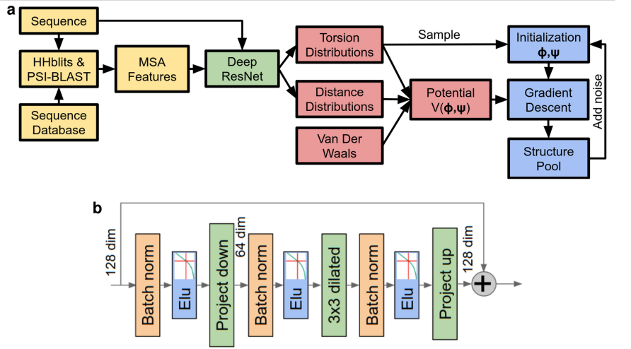
Sequence 입력: 예측하고자 하는 단백질의 아미노산 sequence를 입력
HHblits를 사용한 MSA 생성 및 HMM Profile 생성:
HHblits는 입력된 sequence를 사용하여 sequence database를 검색하고, homologous sequence들을 찾아 
Multiple Sequence Alignment (MSA)를 생성


HMM Profile : 아미노산 발생확률, insertion/deletion 확률


PSI-BLAST를 사용한 Profile Features 생성:
PSI-BLAST는 HHblits가 생성한 MSA, 또는 입력 sequence를 사용하여 Position-Specific Scoring Matrix (PSSM)를 생성
PSI-BLAST는 PSSM을 기반으로 반복적인 검색을 수행하여, 더 멀리 떨어진 homologous sequence까지 찾아내고, PSSM을 업데이트
최종적으로 업데이트된 PSSM으로부터 position-specific substitution probabilities를 추출하여 profile features를 생성


Non-gapped Profile 생성:
HHblits가 생성한 MSA에서 gaps (insertion 또는 deletion)를 제거하고, 각 위치의 아미노산 빈도를 계산하여 non-gapped profile을 생성


Sequence-length Features 생성:
One-hot encoding of amino acid type, deletion probability, residue index 등 sequence 자체의 정보를 나타내는 features를 생성
(이들은 별도의 tool을 사용하지 않고, sequence와 MSA 정보를 바탕으로 직접 계산.)

그 후 입력을 Deep ResNet 을 통해 Torsion Distributions, Distance Distributions, Van Der Waals 를 예측한다. 

잔기별 비틀림 각도는 가능한 각도들의 확률 분포 형태
Distogram은 단백질 내의 모든 아미노산 잔기 쌍 (i, j) 사이의 거리에 대한 확률 분포
AlphaFold는 Rosetta라는 프로그램의 Vscore2_smooth라는 함수를 사용하여 반 데르 발스 상호작용을 고려



그 후 
Potential V(φ, ψ) 생성:

Distogram -> 거리 포텐셜(distance potential) 계산
Torsion Distributions -> 비틀림 각도 포텐셜(torsion potential) 계산
Vscore2_smooth -> Van Der Waals 항 계산
위 세 가지를 합쳐 최종 포텐셜 V(φ, ψ) 생성

그걸 최소화하는 방향으로 학습